The GUI will try to convert old .adf files to new .ams files as best as it can.
We attempt to keep the 2020 GUI version as much backwards compatible as possible for visualizing results such as spectra, orbitals, band structures, trajectories etc. from older .t21 and *kf files.
Please let us know at support@scm.com with your old input / result files if it doesn’t work for you.
In general, the best hardware will be: the latest generation of processors, 4GB RAM per core and an SSD. See also the summary of a hardware FAQ session from October 2020. For the latest information, see our installation manual.
Based on your budget, an older processor, 2GB of RAM per core and a standard hard drive may also be sufficient for running ADF jobs. Since floating-point performance is crucial for ADF, we do not recommend to use hyperthreading or use all Opteron logical cores (i.e. run one process per floating point unit).
Note that since chips are continuously improved, specific recommendations may change. As of mid-2017, these configurations should give the best performance for ADF:
Desktop or laptop: an Intel i7 processor from the latest generation, 16GB of RAM or more, and an SSD (a fusion drive may also work).
High-end workstation or a cluster: a dual-CPU Xeon SP setup with at least 2GB, but better 4GB, of RAM per core and an SSD. Using an SSD becomes more essential as the number of cores per node increases. For calculations on multiple nodes, get a fast interconnect (Infiniband).
Update mid-2019: Rome, the latest Zen 2 AMD architecture (Epyc, 3rd generation Ryzen), give very good performance for ADF. 4GB RAM per core and SSD are still recommended. Make sure you download the Linux binaries optimized for AMD Zen.
Similar requirements should hold for BAND (maybe you can benefit from even more disk space) and ReaxFF (less memory intensive than ADF).
If you open AMS for the first time from your applications, you’ll see a notice “AMS20xx.xxx” can’t be opened because Apple cannot check it for malicious software.
To fix this:
– In the Finder on your Mac, locate the app you want to open.
– Control-click the app icon, then choose Open from the shortcut menu.
– Click Open.
The app is saved as an exception, and you can open it in the future by double-clicking it or from your Applications on the Dock.
Yes! From on AMS2019.304 you can use software rendering instead.
To activate the software rendering, type the following command in your command line before starting the GUI:
export SCM_OPENGL_SOFTWARE=1
To make this permanent, just add it to your $HOME/.bashrc file.
Note: This option replaces the former
export SCM_OPENGL1_FALLBACK=1
Users with older versions can still make use of the old – less efficient – OpenGL 1.4 fallback option, as described in AMS2019/18 or ADF2017.
Please contact support@scm.com if none of the above solves the issue.
In AMS2020 a major overhaul of the input for ADF has been made, unifying inputs more strongly across modules in the suite.
With the restructuring of our code base and introduction of the AMS driver we have rewritten the input handling to improve cross-engine compatibility.
In most cases, the GUI will have backwards compatibility. And so will amsprep and amsreport scripting tools. However, if you use command line input files and home-grown scripts, you will find that unfortunately these will no longer work with our 2018 version.
Starting with AMS2018, just click help -> Command-line (Windows) or Terminal (MacOS) in any GUI window to start a terminal with all the environment variables set properly.
2017 and earlier versions
On Windows, use the adf_command_line.bat tool to open up a command line with the ADF environment set up. You can use ‘sh’ to run a shell command or by itself to open a rudimentary shell.
On a Mac open a terminal and type a dot. Then open a GUI and go to Help: Show AMSHOME in Finder in the menu, drag that to the terminal and press enter (see also video).
Yes, the integrated GUI works with all our software as well as with MOPAC and Quantum ESPRESSO for which also provide binaries.
The GUI used unicode characters in many places. For example, the proper characters for Angstrom, degrees Celcius, and many more. You can see examples by starting AMSinput, selecting a Geometry Optimization, and then going to the details page (by clicking the … button). There you should see a couple of Angstrom symbols if everything is working as intended.
On most machines this will just work out of the box. If not, the issue might be that the default font on the machine does not support such characters. Try installing a font line DejaVU Sans and Monospace DejaVu. On CentOS you can do this (as root) with the command:
yum install dejavu-sans-fonts dejavu-sans-mono-fonts dejavu-serif-fonts
No, usually you don’t need the source code.
We collaborate with all major hardware vendors to port and optimize our code on the most popular platforms. The binaries work out-of-the-box in parallel with fast interconnects through included MPI libraries or with the native parallel libraries (MPT, POE). The binaries are also shipped with linked-in mkl libraries, and are thoroughly tested against a test set before they are released.
Should the latest binary for your system not be available, we are happy to help you port it to your platform. If you are an experienced system administrator you can also compile AMS yourself e.g. on an unusual supercomputing platform. In this case we do not charge you for using the source code.
Only when you want to modify the source code to use non-standard options and features do you need to purchase the source code. Changes in the compiler flags, which have been carefully optimized for performance and robustness, are not recommended and the use of different compiler flags is at your own risk.
Scientists interested in further developing the Amsterdam Modeling Suite should e-mail us to discuss a possible collaboration with SCM, including a discounted (source code) license.
Customers recommend us for the level of support and expertise of our staff. At SCM, the people developing the code are the people giving technical support.
This includes all technical aspects related to installation and bugs, and we sometimes also give some more scientifically oriented help. The latter is done only at SCM’s discretion and is not included in the official standard support.
While we sometimes like to help inexperienced users to get started, we do expect researchers to get a grasp of the theoretical methods and relevant literature.
We cannot guarantee to fix a particular problem or answer any question, but we will do our best to help you!
Hyperthreading does not speed up your ADF (or BAND, DFTB, ReaxFF) calculations, so it is not recommended to enforce this (by using a license for more cores and setting NSCM to double the number of physical cores). For licensing purposes, we only count physical cores. So, for instance, a hexa core machine with hyperthreading counts as six cores.
The Bulldozer-family of AMD architectures (Bulldozer, Piledriver, Steamroller) have only one floating point unit per two cores (module). It is thus recommended to run ADF only on half of the cores on these machines, and we try to license these machines accordingly.
For the AMD Zen generation CPUs (Ryzen/Threadripper/Epyc) ADF should run on all physical cores (without hyperthreading). Linux users should install the AMS2019 Zen binaries, which have been optimized for this CPU architecture.
By default the Amsterdam Modeling Suite and its engines try to use all physical cores. So no hyperthreading and half of the cores of the some AMD architectures.
To change this behavior, you need to set the NSCM variable, either in the environment, in your submit script, or in the queue definition in AMSjobs.
E.g. running from the command line on Linux: export NSCM=4 will make ADF and other modules use 4 cores even if there are 2 or 8 physical cores.
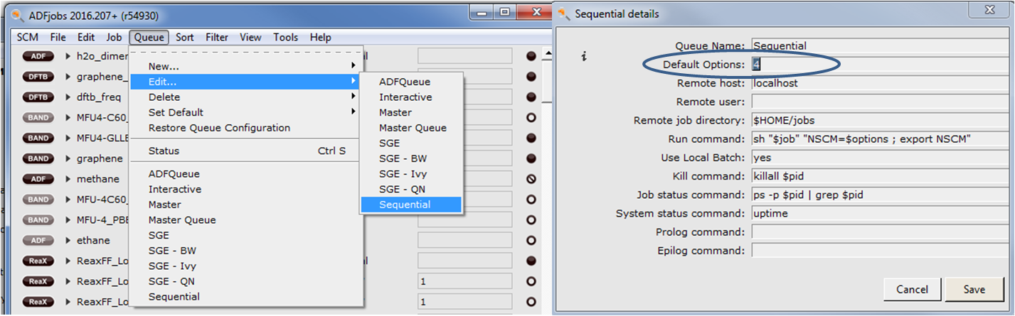
Likewise in AMSJobs you can change your sequential queue Queue => Edit => Sequential
Enter the desired number of cores in the ‘Default Options:’ field. Since this is the default queue so if you run a job without specifying a queue or modifying the default field in AMSJobs, it will use your indicated number of cores.
MPI Application rank … exited before MPI_Finalize() with status …
is an error that could have occurred for several reasons. Please contact support@scm.com with:
- input (.run), output (.out), logifle (.log, error (.err) for your job
- your operating system (Windows 32/64 bit, Linux (distribution), MacOS (version))
- which version of AMS you downloaded
It is easy to have your local GUI to set up and monitor jobs as well as visualize results, while submitting jobs to remote queues.
A video shows how to set up remote queues on Windows.
There are some conditions that must be fulfilled however. The main condition is that you must be able to log on to the remote computer using ssh (or, on Windows, plink.exe) without being asked for any passwords or confirmations. The common way for this is using public key authentication and the ssh-agent. Detailed instructions for Windows users are available in the Readme.rtf document and in its PDF version DocInstallation_windows.pdf (both in the AMS installation folder). Unix/Linux users probably already know how to do this. The other condition is: AMS must be installed on the remote machine and the commands that set up relevant environment variables must be present in the shell profile file, for example ~/.profile.
Suppose you are able to log on to the remote machine and suppose the machine is called cluster.example.com, and your login there is myname (of course you will use real values instead of these). The machine is a login node of a cluster and PBS is the batch system used on the cluster. Our experience shows that this is a very common configuration among AMS users.
Now we need to configure a new queue in AMSjobs. Let’s call the queue cluster_PBS. Use the menu command Queue->;New…->PBS. The template already supplies some default values but you may want to change them depending on the cluster policies.
First the easy parts: type cluster_PBS in the Queue Name field, cluster.example.com for Remote host, myname for Remote user. The Remote job directory specifies a directory on the cluster where AMSjobs will place job files.
The Run command is probably what you will want to think about more thoroughly. In the template it contains
qsub -lnodes=2:ppn=2:infiniband -lwalltime=$options “$job”
You may have to change everything between qsub and “$job” on the line depending on how PBS is configured on the cluster. This will also determine the value for the Default Options entry.
In the template, the wall clock time is configurable per job but you may decide that it is better to have the number of nodes as an option. In this case the Run command will look as:
qsub -lnodes=$options:ppn=2:infiniband -lwalltime=100:00:00 “$job”
Of course you can add there other qsub command line switches that you would normally put in the script after #QSUB. So if you choose to “hard-code” the number of nodes and leave walltime configurable then you may want to name the queue something like cluster_PBS_2nodes. If you choose to hard-code the walltime and leave the number of nodes configurable then you may want to name the queue cluster_PBS_100hr or something like that so that you can distinguish it from other similar queues that differ from this one by the hard-coded value.
After you’ve finished configuring the queue, press Save and test that you can see the status of the queue by selecting menu Queue->Status. This will query the status for each queue defined in AMSjobs by running the command specified in the System status command field (remotely if necessary). If you do not get the queue status but something like “Connection refused” or “No more authentication methods left” then check the ssh connection to the remote computer.
Finally test your queue by running a Test job.
If everything works as you like, you may consider setting your new queue as the Default Queue in AMSjobs. Then using the Run command in AMSinput or in AMSjobs will automatically assign this new queue to your job, and run the job on the remote machine.
This is error is caused by the GUI trying to use the packaged libstdc++, which is older and incompatible with your system libstdc++ needed for your graphics drivers.
The solution is to move the packaged libstdc++. This is done with:
mkdir $AMSBIN/libold
mv $AMSBIN/lib/libstdc++* $AMSBIN/libold/
From AMS2022 onwards this issue is solved with a dependency checker.
In our AMS2020 release, ADF has been fully integrated to the AMS driver, simplifying the input. If you run through the GUI this will not affect you. If you use your own command line input with scripts, your old inputs are not compatible with AMS2020 or beyond. Old ADF inputs can be converted with a simple tool. Let us know at support@scm.com with your old input if that does not work.
No, Gaussian-type orbitals can not be used in ADF, since ADF uses Slater Type Orbitals (STOs).
Slater orbitals are better from a theoretical point of view since they have the correct behavior near the nucleus (cusp) and the correct asymptotic long-range behavior. Consequently, typically fewer STOs than GTOs are needed to reach a certain level of accuracy, as discussed in this news item Slaters beat Gaussians and a paper benchmarking DFT methods for a catalytic reaction.
There is no silver bullet. Some general recommendations follow below, which are by no means definite. Please check the literature carefully and check the robustness of the results by using a large basis set eventually, if possible.
The nomenclature of the STO basis sets in ADF: D, T, and Q stand for double, triple, and quadruple, and (n)P stands for n polarization functions. For example, the DZP basis has double zeta + 1 polarization function. Inner electrons of (atomic) fragments can be frozen during the molecular calculation, this is denoted with ‘small’, ‘medium’ or ‘large’, or by specifically specifying up to which shell the electrons are frozen. In general, we recommend the use of frozen core basis sets for LDA and GGA functionals if available.
All electron basis sets are required in case of SAOP, meta-GGA and meta-hybrid functionals, functionals that use LibXC, post-KS calculations like GW, RPA, MP2 or double hybrids. For hybrid functionals, the use of frozen cores usually is fine for geometries and non-core spectroscopic properties.
There are also specialized basis sets, e.g. containing diffuse functions (“AUG”, for describing anions and diffuse excitations), even-tempered basis sets (“ET”, for describing core electron binding energies), and optimized for ESR A-tensor and NMR spin-spin coupling calculations (ZORA/QZ4P-J). See also the documentation for more technical details and the basis set database in ADF.
The DZP basis set could be a good starting point, especially for geometry optimization. See also this paper looking at catalytic reactions. In general, this basis it is expected to be slightly better than the often used 6-31G* basis set in codes which use Gaussian basis sets. The DZP basis defaults to TZP for transition metals. The frozen core approximation generally does not affect geometries much, but a too large frozen core can lead to inaccuracies.
For the most accurate predictions of spectroscopic properties, the largest QZ4P basis is recommended, although often the TZ2P basis is already close to the basis set limit. Also, usually an all-electron basis set is necessary to properly describe properties related to inner electrons (NMR, EPR, X-ray absorption).
The tutorial on calculating UV/VIS spectra with ADF will get you started with the basics. For getting more accurate results, however, you need to consider the technical details used in TDDFT, such as basis set, exchange correlation functional, and other settings.
There are faster approximate TDDFT methods available, such as TDDFTB (see tutorial), sTDDFT, POLTDDFT and TDDFT+TB (see webinars on the latter).
We also have an advanced tutorial / case study on TDDFT methods.
One can also go beyond TDDFT using quasiparticle self-consistent GW with the Bethe-Salpeter Equation (qsGW-BSE), which could be the most accurate approach.
You are advised to check the literature on which approaches are suitable for similar compounds. Here are some general recommendations on what could work well in ADF:
1) optimize your molecule. Scalar relativistic, TZP, small core (although a large frozen core could also work), and numerical quality ‘Normal’ would typically be quite accurate. As to the functional, a GGA perhaps with dispersion corrections could give very good results (e.g. PBE-D3(BJ)). GGAs are much faster in ADF and can yield better geometries than hybrids. Note that the dispersion interactions affect the geometry, and thereby indirectly the electronic structure, including excitations.
2) TDDFT calculation for UV/VIS. Scalar relativistic up to 4d-elements is usually sufficient. For heavier elements you may want to check the effect of spin-orbit coupling on the spectrum (see also highlight on conversion efficiency of solar cell dyes). You may want a larger basis set (e.g. TZ2P) and perhaps all-electron. Also a higher accuracy may be desirable (good, or excellent). As to the number of excitations, this depends a bit on the electronic ground state and which excitations you are interested in. You could start with 30 or so to see how much to the blue/UV will be covered. Finally the functional could play an important role. The asymptotically correct SAOP model potential is often used, since this is an accurate Kohn-Sham potential well suited to describe virtual orbitals (see publication by Baerends et al.). You could also try hybrids (e.g. B3LYP) or metahybrids (M06-2X). Range-separated hybrids (CAMY-B3LYP) are sometimes advised for excitations with long-range charge transfer character (you can also tune range-separated hybrids). SAOP calculations will be much faster in ADF than hybrids.
Further comments:
- for symmetric systems, ALLOWEDONLY can reduce the computation time by excluding the excitations which are symmetry-forbidden
- for very large systems you may consider trying out TD-DFTB in combination with filtering out the single orbital transitions with very low oscillator strength
- vibronic fine structure may be included by calculating Franck-Condon Factors. Since this involves calculating excited state frequencies (numerically), the calculations can be very demanding for large systems
See also the example on relativistic NMR calculations. Perhaps the unique capabilities of ADF to analyze orbital contributions to NMR are of interest, too.
We also have a tutorial on how to visualize spin-spin coupling.
An all-electron basis set of TZP or higher. TZ2P is usually a good choice. For heavy metals you may consider the ZORA/TZ2P-J or ZORA/QZ4P-J basis.
PBE0 is often a good functional for NMR. If you can’t afford hybrids you could try PBE or SAOP.
For the relativistic approach we recommend at least scalar ZORA. Spin-orbit (SO) ZORA should be used if you are looking at the shift of an heavy atom, or a light atom near a heavy atom.
If SO effects are large, a QZ4P or QZ4P-J basis will improve the description of the induced spin density on the probe nucleus. You may also want to try out the ‘fxc’ kernel option – note that this has a small gauge dependency.
The numerical accuracy should be better than default. You could try NUMERICALQUALITY good or verygood to set the grid and density fitting accuracy.
Disclaimer: These general recommendations are based on the work of Jochen Autschbach‘s group. You should always carefully try out a few different options to test the sensitivity of the DFT methods on the NMR predictions for your own system. Some suggested references:
http://dx.doi.org/10.1002/chem.201502346
http://dx.doi.org/10.1021/ja3040762
http://dx.doi.org/10.1002/anie.201005431
Finding a Transition State (TS) can be difficult. Two things will help the TS search:
- Get a geometry close to the TS
- Get a reasonable Hessian (energy curvature)
1. to get a reasonable starting geometry you could e.g. start with a linear transit, nudged elastic band or from a previous TS geometry of a similar reaction.
2. defining the reaction coordinate (TSRC) may be the easiest option to get a reasonable Hessian. You could also calculate the full Hessian (frequency calculation), a partial Hessian (see BAND tutorial) or a Mobile Block Hessian, which should be better-conditioned.
For all initial Hessian calculations you could consider using a lower-accuracy method (e.g. lower integration accuracy, smaller basis sets, or even using DFTB). You should however always check the Hessian, e.g. by visualizing the frequencies, to check if it has one single negative eigenvalue and whether that eigenmode corresponds to your reaction. For the TS search itself you should switch to higher accuracy – especially think about the numerical integration and density fitting.
See also Tips, tricks, examples and exercises for finding Transition States (pdf, input files)
You can do COSMO calculations with ADF. The COntinuum SOlvation MOdel treats the solvent as a polarizable continuum. You can also use other solvation models (SM12, SCRF, 3D-RISM) or subsystem DFT (Frozen Density Embedding) to include environment effects.
COSMO-RS (Realistic Solvents) is for calculating thermodynamic properties of (mixed) fluids. It uses post-ADF results (sigma profiles) for determining interactions between species in the liquid phase. You will typically not need COSMO-RS if you want to include solvent effects in your DFT calculation, but some properties such as solvation free energies may be more accurately treated with COSMO-RS than with COSMO.
To speed up a molecular or periodic DFT calculation, inner electrons of atoms can be frozen. Note that this is not a pseudopotential: all electrons are still present, the cores are just frozen at their optimized atomic configuration. The effect on the equilibrium geometry and properties of valence electrons is usually small. For spectroscopic properties of core electrons, or electrons close to the nucleus, typically an all electron (AE) approach is necessary.
In the atomic database (you can browse $AMSHOME/atomicdata to see which basis sets are available) the AE basis sets are denoted as the element names, while the name is extended with the highest shell that is kept frozen for the frozen core basis sets.
small core: the smallest core available in the basis set database, for example:
- Rh.3d: all 28 electrons up to 3d are frozen: [Ar]3d10. The valence orbitals are: 4s, 4p, 5s, 4d, 5p.
- Au.4d: all 46 electrons up to 4d are frozen: [Kr]4d10. The valence orbitals are: 5s, 5p, 6s, 4f, 5d, 6p.
large core: the largest core available in the basis set database, for example:
- Rh.4p: all 36 electrons up to 4p are frozen: [Kr]. The valence orbitals are: 5s, 4d, 5p.
- Au.4f: all 60 electrons up to 4f are frozen, [Kr]4d104f14. The valence orbitals are: 5s, 5p, 5d, 6s, 6p.
Note that for some elements and basis sets there is just 1 core available (e.g. 1s for C), in which case all core options default to that specific frozen core.
When there are two options available (e.g. Rh.3d and Rh.4p), the medium core option typically defaults to the large core option. The use of medium core is therefore not recommend, we suggest to choose your specific basis set, either from the GUI in the basis set details panel, or by browsing the available basis sets and specifically defining the appropriate core.
In 2018 a few keywords changed their format and input parsing was made more strict. See the input parsing in the ADF documentation.
Fragment files in ADF no longer need to be spin-restricted. So as of ADF2019, you can use restricted fragments.
No, when you do a spin-restricted calculation in ADF with an odd number of electrons, you do not get the energy expression that is used in ROKS. In ROKS, the spin-unrestricted energy is optimized with alpha orbitals restricted to have the same spatial form as the beta orbitals. In ADF using a restricted calculations with an odd number of electrons will just result in fractional occupations of the frontier orbital. The energy of this electronic configuration is not the same as in a ROKS calculation.
Unrestricted calculations (UKS) in ADF should lead to proper integer occupations of the alpha and beta electrons, which are treated independently and can have spatially different forms.
You can for certain types of calculations (energies, forces and Hessians for GGAs only).
You will need a Linux OS with an NVidia CUDA GPU that does double precision, see the documentation for more details.
ADF does not calculate total energies. It calculates difference energies with respect to fragment energies. By default, these are the spherical spin-restricted atoms. For this reason total energies from other programs cannot be compared to ADF directly. Only energy difference comparisons are meaningful. These are the only energies that play a role in chemistry of course.
If you do need the total energy, there is a workaround: calculate total energies of the atomic fragments and add them to the bonding energy.
Because the total energy of an atom is, by definition, the energy difference between the atom and the (nucleus+free electrons) system one can calculate it by calculating a single atom with the charge equal to the number of electrons. The ‘bonding energy’ of such an ‘atom’ will then be equal to negative of the total energy of the atomic fragment. Care should be taken to apply this trick to frozen-core fragments. In this case, it only makes sense to remove the valence electrons and leave the frozen core.
You need to subtract the bonding energies of the individual atoms from the bonding energy of the molecule.
Care must be taken to get the correct atomic reference state. Usually you will need to break the symmetry (otherwise spherical symmetry is used) and note that ADF can not perform restricted open-shell Kohn-Sham (ROKS) calculations. An example input for the triplet oxygen atom:
System
Atoms
O 0.0 0.0 0.0
End
End
Task SinglePoint
Engine adf
Relativity
Level None
End
SpinPolarization 2
Unrestricted Yes
Basis
Type QZ4P
Core None
End
IrrepOccupations
A 5 // 3
End
numericalquality good
symmetry nosym
xc
hybrid B3LYP
End
EndEngine
There are a few options to aid SCF convergence:
- modern SCF algorithms: A-DIIS is usually a good option, and is default since ADF2016. Alternative options are LISTi (with good scaling) and ARH (slower per SCF cycle). E-DIIS is similar to A-DIIS but slower
- use the OCCUPATIONS key to specify occupation numbers
- use electron SMEARING for systems with low HOMO-LUMO gap
- use KEEPORBITALS to keep the same orbitals occupied after a certain number of steps
See the SCF troubleshooting section of the ADF manual and send us relevant input and output if you keep having problems.
There may be a few reasons why imaginary frequencies are found after geometry optimization:
- Visually inspect the negative normal mode in AMS Spectra by selecting it. Pause at some frame to get the distorted structure, and use Play -> Update geometry in input to use that as a new starting point for geometry optimization. If it’s a frustrated rotation, you can also in the GUI manually distort it by changing the dihedral.
- The optimization threshold is not strict enough for the molecule’s potential energy surface (PES). For example, if there are almost no-barrier rotational modes (e.g. methyl groups in some situations) or cyclopentane-like fragments, then the PES in such cases may be almost flat. In this case, much more strict convergence criteria (and higher integration accuracy) may be necessary to get to the energy minimum.
- Even with tight convergence criteria, one may get a small imaginary frequency due to numerical noise, which is always present in every calculation. In this case, it may be useful to scan the normal mode corresponding to the imaginary frequency and recheck is the frequency is indeed imaginary by finite differences. The latter is done using the SCANFREQ keyword, which is enabled by default in the AMSinput GUI module.
- If the scan shows an imaginary frequency, then it means that the preceeding geometry optimization converged to a saddle point. This may happen when optimization was started close to the saddle point without a good Hessian estimate. In such a case, ADF did not make enough steps to get a good Hessian approximation and figure out that it has negative eigenvalue(s).
Yes, it is be possible to combine COSMO and TDDFT. This will modify the zeroth-order KS orbitals and their energies, which is usually the most important solvation effect. COSMO could also modify the first-order change in the KS potential. This effect has been implemented and will certainly be important in case of a high value for the dielectric constant. The response of the COSMO surface charges due to the TDDFT-induced modified charges may be switched off (NOCSMRSP), which is probably a better representation of the solvent response for instantaneous (de)excitation.
In the response part of the calculations, one can also use a different dielectric constant . The reason for using two different dielectric constants is that the electronic transition can be so fast that only the electronic component of the solvent dielectric can respond, i.e., one should use the optical part of the dielectric constant. This is typically referred to as non-equilibrium solvation. If one optimizes an excited state, the solvent dielectric has time to fully respond and the same dielectric constant should be used..
Yes. See the tutorial and documentation on excited state geometry optimizations.
Yes, this can be done numerically by distorting the structure along the normal modes.
First calculate the normal modes “q” with ADF. Then calculate the polarizability tensor by applying finite electric fields at the geometries q_o + dq and q_o – dq.
From this one can obtain, by double finite difference, the derivative of the polarizability w.r.t. a particular normal mode of interest. This should be less time-consuming then a regular Raman calculation as well.
The beta tensor can be obtained by using the input key RESPONSE, for example:
RESPONSE
HYPERPOL 0.03
 DYNAHYP
 ALLCOMPONENTS
 END
In order to obtain gamma, one should calculate beta in small electric fields. Such a field can be switched on by specifying, for example: EFIELD 0 0 0.001 for an electric field of 0.001 a.u. in the z-direction. The beta calculation needs to be repeated for different field directions. gamma_zzzz can be obtained from (for example): gamma_zzzz = beta_zzz (E=0.001 z) – beta_zzz (E=-0.001z) / (2 * 0.001)
Similar relations hold for other tensor components.
Recently, the group of Lasse Jensen has implemented damped quadratic and cubic response, which gives access to many non-linear optical properties including two-photon absorption. These methods will become available in ADF2017.
For a spin restricted open-shell calculation, save TAPE21, and use the whole molecule as a fragment in a SR unrestricted calculation with the keywords:
scf
iter 0
end
ADF wil use the fragment density coming from the spin-restricted calculation as start-up density in the unrestricted calculation. iter 0 means that only 1 scf-iteration will be performed with the use of the fragment density (one should use the same XC-potential in both calculations of course), such that the alpha-orbital energies remain degenerate with the beta-orbitals.
After a calculation with ADF, BAND, ReaxFF, DFTB etc you will have a result file (a .t21, .runkf, .rxkf, or .rkf file). These are binary files, and like all other binary files used by the ADF package they are written using the KF library. The data are organized in sections, and each section can contain variables (either real, integer, string or logical). They may be transported between different platforms, conversion is performed automatically when needed.
Not all data on the files are intended to be used directly by end users, the detailed meaning of many data items will not be clear to end users who do not have access to the source code. Preferably use the GUI utilities to visualize the results or scripting tools to get relevant results from a batch of calculations.
The KF Browser is a useful tool to browse through our binary files. The available data can be searched, copied as text and plotted as graphs. It can be started from the GUI (SCM → KF Browser) or from the command line ($ADFBIN/kfbrowser filename). To see all raw data, switch to the Expert mode (File → Expert Mode in KF Browser).
adfreport is a command line tool to quickly access results from different result files (.t21, .runkf, .rkf, .rxkf) in a uniform manner. You can get any variable from a result file by key value, or you can use predefined report commands (like geometry, charges, energy, etc). Run with the -h flag to get help and a detailed description of all predefined commands).
Note: if you include the -h flag and a filename, you will get specific help for the contents of that file.
To use adfreport via the command line: $ADFBIN/adfreport [-h] filename
KF Utilities are a set of command line utilities to handle KF files.
pkf: print the table of contents
dmpkf: dump the contents of all or part of a KF file to an ASCII file
udmpkf: make a binary KF file out of a ASCII file (typically a dumped KF File)
cpkf: copy all or part of one KF file to another KF file, or remove data from a KF file.
KFReader: C routines to read binary KF files
kf.py: python interface for reading binary KF files (requires ADF installation).
A possible origin of this problem is that ADF symmetrizes the input coordinates of fragments which are nearly symmetric. As a consequence, the fragment coordinates can no longer be transformed to their position in the full calculation of the complex.
The workaround is to use SYMMETRY TOL=1.0e-10 in the calculation of the fragments, such that the coordinates in the fragments are not symmetrized.
This message shows that the numerical integration is not as accurate as required (currently tested only with spin-orbit calculations). You can force the calculation to continue using the ALLOW BADINTEGRALS input key. This will force the calculation to continue, but remember there are possible inaccuracies due to these integrals. You can probably increase the accuracy of the eta integrals by increasing the overall integration accuracy (using the integration key). One will then probably still get the BAD ETA INTEGRALS message, but this is relative to the required accuracy. One can check the accuracy (it is printed on output), and if the accuracy is good enough one can use the ALLOW BADINTEGRALS key to force the calculation to continue.
One of the reasons can be that the SCM_TMPDIR environment variable also contains non-ASCII characters and ADF cannot use it. The solution is to set the SCM_TMPDIR value to a path that does not contain non-ASCII characters, for example, C:\TMP:
- Right click on My Computer
- Select Properties item in the pop-up menu
- Click on the “Advanced” tab
- Click on the “Environment Variables” button
- In the upper half under “User variables for …”, click the New button
- Enter SCM_TMPDIR in the variable name and C:/TMP in the variable value field. Please note that the path in the variable value must not contain spaces. It is also advised to use forward slashes as a path separator instead of the backslash
- Make sure the C:\TMP directory exists and is writable by anyone
- Click on the Ok button in all windows to confirm your change
- If you use the GUI, restart it so the change takes effect
Most probably you use the INTEGRATION key for a fragment analysis and thereby using an incompatible combination of ZlmFit and Voronoi grid for fragment calculations.
You should either use Voronoi + STOfit or Becke + ZlmFit (which is the default since ADF2014).
Explanation of the terms in the error: “Int. Energy with ZlmFit+LargeFragment+VoronoiGrid not implemented”
1. ZlmFit means the way the Coulomb potential is fitted. ZlmFit is the default in ADF2014 and beyond. One can also use the STOFit, using the key STOFIT. If one would use STOFIT this error would not appear.
2. LargeFragment means a fragment larger than an atom.
3. VoronoiGrid is the integration method. The VoronoiGrid will be used if one is using the INTEGRATION key. In ADF2013 and beyond the Becke grid has become the default. If one would use the default integration method in ADF, which is the BeckeGrid, this error would not appear.
Recommended is to use the BeckeGrid and ZlmFit if one has larger fragments, possibly using quality good.
Amsterdam Modeling Suite (AMS) refers to the whole suite which includes the AMS driver for complex potential energy surface tasks with any underlying engine. The AMS bundle further includes the integrated GUI and the compute engines ADF, BAND, DFTB, MOPAC, ReaxFF, UFF, COSMO-RS.
It’s a driver for running molecular dynamics or exploring the potential energy surface (finding transition states etc.)
It can be used with different modules: ADF, BAND, DFTB, MOPAC, ReaxFF and external engines. And as such you can switch easily between them, e.g. to transfer a Hessian from a low-lying method.
With AMS2018.103 it will exit with an error.
Starting with r69000, AMS geometry optimizations try to continue even if engine fails to solve for a geometry.
This can happen if there are for example SCF convergence problems in the engine. The energy/gradients might then not be quite correct, but it is probably safe to continue the optimization and hope that things are fine again for the next step. Note that this fix also applies to PES scans, transition state searches, and any other applications that use geometry optimizations internally (e.g. elastic property calculations).
BAND does not calculate the total energy. Instead, it calculates the formation energy with respect to the spherically symmetric spin-restricted atoms. The reason is that this number is easier to determine accurately using numerical integration then the total energy.
The problem is that BAND is (internally) centralizing the atom positions with respect to the geometrical center of the structure. During this centralization an atom can be positioned on one side of the unit cell or the other. (the result for this individual calculation will be the same in both cases, but for a PEDA calculation that is not true) In your case, the centralization of the fragments and of the PEDA calculation gave results which cannot be transformed into one another by a simple translation.
The solution is to pre-centralize the whole system with respect to the geometrical center of the “bigger” fragment. (since this fragment usually gives this problem) E.g. if you study a surface-adsorbate interaction, you centralize the whole structure w.r.t. the geometrical center of the surface. In some cases the adsorbate fragment might be the reason of the problem. If so, we recommend redefining the unit cell so that the adsorbate is closer to the center of the unit cell than to any of the borders of the unit cell.
If this approach does not solve your problem please send us your input and output, so we can look into it.
The dimension of the text-book “density of states per unit cell” (DOS) is [1/energy].
What is plotted in the BAND-GUI is not the DOS, but a histogram of the DOS, which is a dimensionless quantity.
The “unit” of the y-axis is [number of states / unit cell].
Each data-point in the plotted DOS represents the number of states (per unit cell) in an energy interval DeltaE. The histogram bin-width DeltaE depends on the DOS input options “Energies”, “Min”, “Max”: DeltaE = (Max-Min)/Energies.
In case one really wants the “text-book” dos, one can set the Dos%IntegrateDeltaE option to “false”. The result will be a very wild function.
The negative values in the partial DOS are artifacts due to the fact that in a non-orthogonal basis set the definition of a “partial DOS” is somewhat arbitrary.
The partial DOS can be a useful tool for understanding the physics/chemistry of your system, but it’s strictly speaking not a “physical quantity”.
Absolute values of orbital energies are physically meaningful for non-periodic systems, 1D periodic systems and 2D periodic systems.
For these cases, E=0 corresponds to the energy of a free electron and the absolute value of the Fermi energy is equal (to a first approximation) to the work function.
In 3D periodic systems the orbital energies (and Fermi energy) are defined up to a constant, ergo the absolute value of energy bands does not have a clear physical meaning (we nonetheless use the convention of setting V_{k=0} = 0, like most other programs).
The DFTB module in the Amsterdam Modeling Suite ships with the following parameters:
- GFN1-xTB: extended Tight Binding parameters for elements H-Rn (all spd elements). Can be used for all properties.
- Quasinano 2013: electronic parameters for H-Po, La, Th. Enabling electronic properties like band structures, DOS, UV/VIS, NEGF
- Quasinano 2015: + repulsive parameters for H-Ca, Br. Enabling geometry optimization, IR spectra, MD.
- Dresden parameters: C, H, O, N, P, S, Al, Si, Ti, Cu, Na, see
$ADFHOME/atomicdata/DFTB/Dresden/README - DFTB.org parameters (see Readme or dftb.org website for latest info). Encrypted parameters may also be evaluated during trial
- Dispersion corrections available (Grimme’s D2 & D3(BJ), London, UFF)
Yes, with DFTB3 and either the Quasinano or the DFTB.org 3ob parameters sets. With other DFTB methods and parameter sets you can use D2, London (ULG) or UFF dispersion.
We have implemented Grimme’s first GFN-xTB method (GFN1-xTB). The second set (GFN2-xTB) usually does not improve accuracy much and has not yet been implemented.
Fields with DFTB are under development. We hope to offer this functionality in our 2020 release.
Yes, DFTB can be applied to 0D systems (molecules), 1D systems (polymers, nanotubes), 2D systems (surfaces), and 3D systems (bulk).
For 1D and 2D systems we have proper periodic boundary conditions. So you do not need to work with large unit cells and slab-gap approximations.
All DFTB parameters can be used for all periodicity.
In AMS2019 we have made a new MOPAC library, which is fully integrated as an Engine with the AMS driver and our GUI. This new MOPAC works much faster as a pre-optimizer and with any AMS driver functionality.
This version of MOPAC is based on the original MOPAC code of Dr. Stewart and contains much but not all of the functionality. In AMS2019, MOPAC is included with the DFTB module.
Older ADF Modeling License suite licenses could also contain the external MOPAC binary and corresponding GUI support.
In ADFInput in the Details → Run script tab, you can change the MOPAC input file before submitting the calculation.
A list of MOPAC keywords (from http://openmopac.net/manual/allkeys.html):
Keywords used in MOPAC2012
| & | Turn next line into keywords |
| + | Add another line of keywords |
| 0SCF | Read in data, then stop |
| 1ELECTRON | Print final one-electron matrix |
| 1SCF | Do one scf and then stop |
| ADD-H | Add hydrogen atoms (intended for use with organic compounds) |
| A0 | Input geometry is in atomic units |
| AIDER | Read in ab-initio derivatives |
| AIGIN | Geometry must be in gaussian format |
| AIGOUT | In arc file, include ab-initio geometry |
| ALLBONDS | Print final bond-order matrix, including bonds to hydrogen |
| ALLVEC | Print all vectors (keywords vectors also needed) |
| ALT_A=A | In PDB files with alternative atoms, select atoms A |
| ALT_R=A | In PDB files with alternative residues, select residues A |
| ANGSTROMS | Input geometry is in Angstroms |
| AUTOSYM | Symmetry to be imposed automatically |
| AUX | Output auxiliary information for use by other programs |
| AM1 | Use the AM1 hamiltonian |
| BAR=n.nn | reduce bar length by a maximum of n.nn% |
| BCC (Unique) | Solid is body-centered cubic (used by BZ) |
| BFGS | Optimize geometries using bfgs procedure |
| BIGCYCLES=n | Do a maximum of n big steps |
| BIRADICAL | System has two unpaired electrons |
| BONDS | Print final bond-order matrix |
| BZ | Generate a file for use by program BZ |
| CAMP | Use Camp-King converger in SCF |
| CARTAB | Print point-group character table |
| C.I.=n C.I.=(n,m) |
A multi-electron configuration interaction specified |
| CHAINS(text) | In a protein, explicitely define the letters of chains. |
| CHECK | Report possible faults in input geometry |
| CHARGE=n | Charge on system = n (e.g. NH4 = +1) |
| CHARGES | Print net charge on system, and all charges in the system |
| CHARST | Print details of working in CHARST |
| CIS | C.I. uses 1 electron excitations only |
| CISD | C.I. uses 1 and electron excitations |
| CISDT | C.I. uses 1, 2 and 3 electron excitations |
| COMPFG | Print heat of formation calculated in COMPFG |
| COSCCH | Add in COSMO charge corrections |
| COSWRT | Write details of the solvent accessible surface to a file |
| CUTOFP=n.nn | Madelung distance cutoff is n .nn Angstroms |
| CUTOFF=n.nn | In MOZYME, the interatomic distance where the NDDO approximation stops |
| CYCLES=n | Do a maximum of n steps |
| CVB | In MOZYME. add and remove specific bonds to allow a Lewis or PDB structure. |
| DAMP=n.nn | n MOZYME. damp SCF oscillations using a factor of n.nn |
| DATA=text | Input data set is re-defined to text |
| DCART | Print part of working in DCART |
| DDMAX=n.nn | See EF code |
| DDMIN=n.nn | Minimum trust radius in a EF/TS calculation |
| DEBUG | Debug option turned on |
| DEBUG PULAY | Print working in PULAY |
| DENOUT, DENOUTF | Density matrix output |
| DENSITY | Print final density matrix |
| DERI1 | Print part of working in DERI1 |
| DERI2 | Print part of working in DERI2 |
| DERITR | Print part of working in DERIT |
| DERIV | Print part of working in DERIV |
| DERNVO | Print part of working in DERNVO |
| DFORCE | Force calculation specified, also print force matrix. |
| DFP | Use Davidson-Fletcher-Powell method to optimize geometries |
| DISEX=n.nn | Distance for interactions in fine grid in COSMO |
| DISP | Print the hydrogen bonding and dispersion contributions to the heat of formation |
| DMAX=n.nn | Maximum stepsize in eigenvector following |
| DOUBLET | Doublet state required |
| DRC DRC=n.nnn |
Dynamic reaction coordinate calculation |
| DUMP=nn.nn | Write restart files every n seconds |
| ECHO | Data are echoed back before calculation starts |
| EF | Use ef routine for minimum search |
| EIGEN | Print canonical eigenvectors instead of LMOs in MOZYME calculations |
| EIGS | Print all eigenvalues in ITER |
| ENPART | Partition energy into components |
| EPS=n.nn | Dielectric constant in COSMO calculation |
| ESP | Electrostatic potential calculation |
| ESPRST | Restart of electrostatic potential |
| ESR | Calculate RHF spin density |
| EXCITED | Optimize first excited singlet state |
| EXTERNAL=name | Read parameters off disk |
| FIELD=(n.nn,m.mm,l.ll) | An external electric field is to be used |
| FILL=n | In RHF open and closed shell, force M.O. n to be filled |
| FLEPO | Print details of geometry optimization |
| FMAT | Print details of working in FMAT |
| FOCK | Print last Fock matrix |
| FREQCY | Print symmetrized Hessian in a FORCE calculation |
| FORCE, FORCETS | Calculate vibrational frequencies |
| GEO-OK | Override some safety checks |
| GEO_REF=<text> | Use native structure as reference |
| GNORM=n.nn | Exit when gradient norm drops below n .n kcal/mol/Angstrom |
| GRADIENTS | Print all gradients |
| GRAPH | Generate unformatted file for graphics |
| GRAPHF | Generate formatted file for graphics suitable for Jmol and MOPETE. |
| HCORE | Print all parameters used, the one-electron matrix, and two-electron integrals |
| HESSIAN | Print Hessian from geometry optimization |
| HESS=n | Options for calculating Hessian matrices in EF |
| H-PRIORITY H-PRIORITY=n.nn |
Heat of formation takes priority in DRC |
| HTML | Write a web-page for displaying and editing a protein |
| HYPERFINE | Hyperfine coupling constants to be calculated |
| INT | Make all coordinates internal coordinates |
| INVERT | Reverse all optimization flags |
| IONIZE | Do not use – use SITE=(IONIZE) instead |
| IRC IRC=n |
Intrinsic reaction coordinate calculation |
| ISOTOPE | Force matrix written to disk (channel 9 ) |
| ITER | Print details of working in ITER |
| ITRY=nn | Set limit of number of SCF iterations to n |
| IUPD=n | Mode of Hessian update in eigenvector following |
| KINETIC=n.nnn | Excess kinetic energy added to DRC calculation |
| KING | Use Camp-King converger for SCF |
| LARGE | Print expanded output |
| LBFGS | Use the low-memory version of the BFGS optimizer |
| LET | Override certain safety checks |
| LEWIS | Print the Lewis structure |
| LINMIN | Print details of line minimization |
| LOCALIZE | Print localized orbitals. These are also called Natural Bond Orbitals or NBO |
| LOCATE-TS | Given reactants and products, locate the transition state connecting them |
| LOG | Generate a log file |
| MECI | Print details of MECI calculation |
| MERS=(n1,n2,n3) | Keyword for BZ |
| METAL=(a[,b[,c[…]]]) | Make specified atoms 100% ionic |
| MICROS=n | Use specific microstates in the C.I. |
| MINMEP | Minimize MEP minima in the plane defined |
| MMOK | Use molecular mechanics correction to CONH bonds |
| MNDO | Use the MNDO hamiltonian |
| MNDOD | Use the MNDO-d hamiltonian |
| MODE=n | In EF, follow Hessian mode no. n |
| MOL_QMMM | Incorporate environmental effects in the QM/MM approach |
| MOLDAT | Print details of working in MOLDAT |
| MOLSYM | Print details of working in MOLSYM |
| MOPAC | Use old MOPAC definition for 2nd and 3rd atoms |
| MOZYME | Use the Localized Molecular Orbital method to speed up the SCF |
| MS=n | In MECI, magnetic component of spin |
| MULLIK | Print the Mulliken population analysis |
| N**2 | In excited state COSMO calculations, set the value of N**2 |
| NLLSQ | Minimize gradients using NLLSQ |
| NOANCI | Do not use analytical C.I. derivatives |
| NOGPU | Do not use GPU acceleration |
| NOLOG | Suppress log file trail, where possible |
| NOMM | Do not use molecular mechanics correction to CONH bonds |
| NONET | NONET state required |
| NONR | Do not use Newton-Raphson method in EF |
| NOOPT, NOOPT-X | Do not optimize the coordinates of all atoms of type X |
| NOREOR | In symmetry work, use supplied orientation |
| NORESEQ | Suppress the default re-sequencing of atoms to the PDB sequence |
| NOSWAP | Do not allow atom swapping when GEO_REF is used |
| NOSYM | Point-group symmetry set to C1 |
| NOTHIEL | Do not use Thiel’s FSTMIN technique |
| NOTXT | Remove any text from atom symbols |
| NOXYZ | Do not print Cartesian coordinates |
| NSPA=n | Sets number of geometric segments in COSMO |
| NSURF | Number of surfaces in an ESP calculation |
| OCTET | Octet state required |
| OLDCAV | In COSMO, use the old Solvent Accessible Surface calculation |
| OLDENS | Read initial density matrix off disk |
| OLDFPC | Use the old fundamental physical constants |
| OLDGEO | Previous geometry to be used |
| OMIN=n.nn | In TS, minimum allowed overlap of eigenvectors |
| OPEN(n1,n2) | Open-shell UHF or RHF calculation requested |
| OPT, OPT-X | Optimize the coordinates of all atoms of type X |
| P=n.nn | An applied pressure of n.nn Newtons/m2 to be used |
| PDB | Input geometry is in protein data bank format |
| PDB=(text) | User defined chemical symbols in protein data base |
| PDBOUT | Output geometry in pdb format |
| PECI | C.I. involves paired excitations only |
| PI | Resolve density matrix into σ, π, and δ components |
| pKa | Print the pKa for ionizable hydrogen atoms attached to oxygen atoms |
| PL | Monitor convergence of density matrix in ITER |
| PM3 | Use the MNDO-PM3 Hamiltonian |
| PM6 | Use the PM6 Hamiltonian |
| PM6-D3 | Use the PM6 Hamiltonian with Grimme’s corrections for dispersion |
| PM6-DH+ | Use the PM6 Hamiltonian with corrections for dispersion and hydrogen-bonding |
| PM6-DH2 | Use the PM6 Hamiltonian with corrections for dispersion and hydrogen-bonding |
| PM6-DH2X | Use PM6 with corrections for dispersion and hydrogen and halogen bonding |
| PM6-D3H4 | Use PM6 with Řezáč and Hobza’s D3H4 correction |
| PM6-D3H4X | Use PM6 with Brahmkshatriya, et al.’s D3H4X correction |
| PMEP | Complete semiempirical MEP calculation |
| PM7 | Use the PM7 Hamiltonian |
| PM7-TS | Use the PM7-TS Hamiltonian (only for barrier heights) |
| PMEPR | Complete semiempirical MEP in a plane to be defined |
| POINT=n | Number of points in reaction path |
| POINT1=n | Number of points in first direction in grid calculation |
| POINT2=n | Number of points in second direction in grid calculation |
| POLAR | Calculate first, second and third order polarizabilities |
| POTWRT | In ESP, write out electrostatic potential to unit 21 |
| POWSQ | Print details of working in POWSQ |
| PRECISE | Criteria to be increased by 100 times |
| PRESSURE | Apply pressure or tension to a solid or polymer |
| PRNT=n | Print details of geometry optimization in EF |
| PRTCHAR | Print charges in ARC file |
| PRTINT | Print interatomic distances |
| PRTMEP | MEP contour data output to <filename>.mep |
| PRTXYZ | Print Cartesian coordinates |
| PULAY | Use Pulay’s converger to obtain a SCF |
| QMMM | Incorporate environmental effects in the QM/MM approach |
| QPMEP | Charges derived from Wang-Ford type AM1 MEP |
| QUARTET | Quartet state required |
| QUINTET | Quintet state required |
| RAPID | In MOZYME geometry optimizations, only use atoms being optimized in the SCF |
| RECALC=n | In EF, recalculate Hessian every n steps |
| RE-LOCAL, RE-LOCAL=n | During and at end of MOZYME calculation, re-localize the LMOs |
| RELSCF | Default SCF criterion multiplied by n |
| REORTHOG | In MOZYME, re-orthogonalize LMO’s each 10 SCF calculations. |
| RESEQ | Re-arrange the atoms to match the PDB convention |
| RESIDUES | Label each atom in a polypeptide with the amino acid residue |
| RESTART | Calculation restarted |
| RHF | Use Restricted Hartree-Fock methods |
| RM1 | Use the RM1 Hamiltonian |
| RMAX=n.nn | In TS, maximum allowed ratio for energy change |
| RMIN=n.nn | In TS, minimum allowed ratio for energy change |
| ROOT=n | Root n to be optimized in a C.I. calculation |
| RSCAL | In EF, scale p-RFO to trust radius |
| RSOLV=n.nn | Effective radius of solvent in COSMO |
| SADDLE | Optimize transition state |
| SCALE | Scaling factor for van der waals distance in ESP |
| SCFCRT=n.nn | Default SCF criterion replaced by the value supplied |
| SCINCR=n.nn | Increment between layers in ESP |
| SEPTET | Septet state required |
| SETPI | In MOZYME, some π bonds are explicitly set by the user |
| SETUP | Extra keywords to be read from setup file |
| SEXTET | Sextet state required |
| SHIFT=n.nn | a damping factor of n defined to start SCF |
| SHUT <file> | Send a command to MOPAC to make a restart and density file, then stop. |
| SIGMA | Minimize gradients using SIGMA |
| SINGLET | Singlet state required |
| SITE=(text) | Define ionization state of residues in proteins |
| SLOG=n.nn | In BFGS optimization, use fixed step of length n .nn |
| SLOPE | Multiplier used to scale MNDO charges |
| SMOOTH | In a GRID calculation, remove artifacts caused by the order in which points are calculated |
| SNAP | Increase precision of symmetry angles |
| SPARKLE | Use sparkles instead of atoms with basis sets |
| SPIN | Print final UHF spin matrix |
| START_RES(text) | Define starting residue numbers in a protein, if different from the default |
| STATIC | Calculate Polarizability using electric fields |
| STEP | Step size in path |
| STEP1=n.nnn | Step size n for first coordinate in grid calculation |
| STEP2=n.nnn | Step size n for second coordinate in grid calculation |
| STO3G | Deorthogonalize orbitals in STO-3G basis |
| SUPER | Print superdelocalizabilities |
| SWAP | This keyword is now obsolete, see NOSWAP |
| SYBYL | Output a file for use by Tripos’s SYBYL program |
| SYMAVG | Average symmetry equivalent ESP charges |
| SYMOIR | Print characters of eigenvectors and print number of I.R.s |
| SYMTRZ | Print details of working in subroutine SYMTRZ. |
| SYMMETRY | Impose symmetry conditions |
| T=n[M,H,D] | A time of n seconds requested |
| THERMO THERMO(nnn) THERMO(nnn,mmm) THERMO(nnn,mmm,lll) |
Perform a thermodynamics calculation |
| THREADS=n | Set the number of threads to be used in parallelization to n |
| TIMES | Print times of various stages |
| T-PRIORITY T-PRIORITY=n.nn |
Time takes priority in DRC |
| TRANS TRANS=n |
The system is a transition state (used in thermodynamics calculation) |
| TRIPLET | Triplet state required |
| TS | Using EF routine for TS search |
| UHF | Use the Unrestricted Hartree-Fock method |
| VDW(text) | Van der waals radius for atoms in COSMO defined by user |
| VDWM(text) | Van der waals radius for atoms in MOZYME defined by user |
| VECTORS | Print final eigenvectors |
| VELOCITY | Supply the initial velocity vector in a DRC calculation |
| WILLIAMS | Use Williams surface |
| X-PRIORITY=n.nn | Geometry changes take priority in DRC |
| XENO | Allow non-standard residues in proteins to be labeled. |
| XYZ | Do all geometric operations in Cartesian coordinates |
| Z=n | Number of mers in a cluster |
Besides facilitating building molecules, our GUI can also visualize the progress of geometry optimizations, MOPAC charges, and IR modes. Geometry optimization can also be done interactively, e.g. to pre-optimize your molecule or periodic system.
In AMS2020, ReaxFF integrated with the AMS driver is the default. This gives consistent input for different modules and enables new properties through the central driver. It also helps users more easily switch between modules and use ReaxFF in multi-layer hybrid simulations.
Some ReaxFF features have not yet been ported to the integrated ReaxFF, and can be used from the standalone ReaxFF.
Click on i next to Force field input in ReaxFF Input to see which force fields are included with ReaxFF. Alternatively, open $AMSHOME/atomicdata/ForceFields/ReaxFF/Readme, which also contains the original references and sometimes a short description. The list of currently available ReaxFF force fields are available in the documentation.
You are strongly advised to check the original publications to see how the force field has been trained and to what type of systems it has been applied.
If no force field is available for your elements, check the literature or parametrize it yourself, see the other FAQs.
This is hard work, which takes quite a bit of training and experience.
The ReaxFF parameters are typically trained against DFT data and parameters should be optimized for all atom types in your system. In principle, parameters are transferable across systems, but including additional atoms requires also to include new interactions with all new element combinations. This is not trivial, but we try to help you with our ParAMS ReaxFF parametrization tools.
RxFF consulting offers consulting services for optimizing force field parameters for new materials.
There are two elements in your simulation box for which no bonded parameters are present in the force field file. Please check the description and the paper on the ReaxFF force field page.
You can find more info on which bond, angle, and dihedral terms exist, and which ones are missing by using the checkreaxffforcefield.py utility:
$AMSBIN/startpython $AMSHOME/scripting/standalone/reaxff/checkreaxffforcefield.py /path/to/yourreaxff.ff
You’ll probably find that this force field was not designed for the elements you want to study. Perhaps there is another force field more suitable for your application.
You may try to our reparametrize the force field.
In the GUI: build a ReaxFF input with these elements X, Y, and Z, and click on the folder icon next to Force field:. A list of force fields included in the AMS/ReaxFF distribution that contain these atom types will be shown. If force fields are available, consult the Readme (click ‘i’) to check the publication to make sure this is the force field for your application.
If no force field shows up in the list, no suitable force field is available in your distribution. Use google or web of knowledge to find out if a ReaxFF force field exists for your application. If it does, and the force field is printed in the supporting information, you can add the ReaxFF force field file (see FAQ) to the existing ones in the distribution.
Note that not all terms may be available for all element combinations. To get more insight in which force field terms are available, use the python ReaxFF force field checking tool:
$AMSBIN/startpython $AMSHOME/scripting/standalone/reaxff/checkreaxffforcefield.py /path/to/yourreaxff.ff
You can find a description of the general structure of the force field file and the parameters from the original ReaxFF documentation.
We try to include as much information on the origin of parameters the ReaxFF manual as well as in the GUI help files.
Many published ReaxFF force fields are building upon a previous set of parameters, and so only the elements studied in that paper are being refined, and the other parameters are just kept in place. You could try to trace back the origin of some of these parameters by looking at the existing force fields and finding out where the same parameters for a particular element also appear. Any force field that has matching atomic parameters might have some information about the origins of the parameters in the corresponding publication or in the information in the force field description file.
However, you need to be careful by just combining and using elements / parameters from different force fields. See also the FAQ about ReaxFF parameter transferability. You should also be aware that certain bonded terms may not be available for a particular unpublished element and/or combination of elements, so you are strongly advised to check this with our ReaxFF force field checking tool: $AMSHOME/scripting/checkreaxffforcefield.py. The original ReaxFF documentation describes the general structure and correspondence of the columns with the parameters.
In general the parameters are quite transferable, but some forcefields were developed for specialized cases such as explosives research (high pressure). It is good practice to scan through the publication of the forcefield (you can find the information by clicking the “i” button behind the forcefield ) before using it extensively. It is also wise to do some testing simulations to see if your structures are not falling apart or folding into weird geometries.
This is most easily done from the GUI using the File → Export Trajectory As: option in AMSJobs. You can export as Gromacs, PDB trajectory, or xmol file. For the .gro export you will get an additional dialogue window where you can include the timestep and the velocities.
Alternatively, you can use the scripting tool amsreport, e.g. amsreport yourreaxff.rxkf -r gro-t0.00025 > yourreaxff.gro
The options for amsreport in your AMS distribution are displayed if you type amsreport -h
During a non-reactive ReaxFF simulation the connection table is determined only once at the beginning of a simulation and is then kept fixed. Other than this the same ReaxFF procedure with the same forces and energy expressions is used. Therefore, if the system is far from equilibrium, or if the temperature is too high, bonds may still be broken or formed.
You can also think about simulating the system at zero Kelvin with a strong thermostat to try and get your system to the nearest local minimum without changing the bonds too much.
This depends on what parameters are available in the force field file. A ReaxFF force field consists of some generic parameters, a number of atomic parameters (1 set for every atom type), bond parameters (combination of 2 atom types), angle parameters (combination of 3 atom types), dihedral parameters (combination of 4 atom types) and possibly hydrogen bond parameters (see original ReaxFF documentation for more details).
If a force field has elements X, Y an Z it means that it contains atomic parameters for X, Y and Z. However, it does not necessarily contain all combinations of the bond/angle/dihedral parameters. For example, X-X, Y-Y, Z-Z, X-Y and X-Z might have bond parameters, but Y-Z could be left out. This means that Y and Z should not be used together in the simulation, as their interaction is not defined.
To get more insight in which terms are available in a ReaxFF force field, use the python ReaxFF force field checking tool: $AMSHOME/scripting/checkreaxffforcefield.py
ReaxFF consists of two parts: the program and the force field files:
– The ReaxFF program is an implementation of the ReaxFF forcefield equations (see the Required citations ReaxFF page for the original papers).
– The ReaxFF force field files contain the parameters needed by the force field equations when running your simulation, they consist of 5 or 6 parts (see original ReaxFF documentation for more details):
* generic parameters
* atom parameters (per element)
* atom pairs / bond parameters (combination of two elements)
* angle parameters (combination of three elements)
* dihedrals (combination of four elements)
* and sometimes hydrogen bonds (per element)
A ReaxFF force field is build using a training set (see other FAQs) and is usually targeted for a specific simulation and typically includes about 4 to 12 elements, as the number of parameters scales to the 4th power with the number of elements included. Because ReaxFF uses pair/angle/dihedral parameters, it is not possible to simply combine two forcefield files.
The AMS GUI can tell you if a force field is available for the elements in your simulation (see other FAQs), but it will not be able to tell if the force field is conditioned for your specific simulation type. For this you will have to check the publication of the force field (doi link is usually included in the Readme file or the first line of the force field file)
The AMS implementation of ReaxFF still takes the original format. If a publication has the parameters printed in the supporting information in native format, just copy that data and save it as a file, e.g. YourNewReaxFF.ff, in $AMSHOME/atomicdata/ForceFields/ReaxFF. Then you can start using that force field by selecting it in the GUI, by clicking other after you’ve clicked the folder icon next to Force field: in the input panel.
If the parameters are printed in tables in the manuscript, but not as a comprehensive SI file, you can still compile your own ReaxFF force field file from this data in the same original ReaxFF format.
It is advisable to use the checkreaxffforcefield.py script in $AMSHOME/scripting/ to check your force field. If you have modified or downloaded a force field you may want to clean it up:
Open a shell in a terminal with AMS settings loaded. Then run the rxffutil tool
rxffutil reformat < your_ff.ff
The resulting cleaned up ReaxFF force field is stored in a file ‘ffield’.
For the NHC themostat/MTK barostat, the simulation samples the correct ensemble no matter what the damping time is set to, but it is recommended to set the damping time to roughly correspond to the correlation time of the system (how long it takes for the system to “forget” a disturbance). This is 2-3 picoseconds in liquid water, up to a couple hundred fs in solids. Setting it any longer doesn’t improve the accuracy of the system anymore, just makes the thermostatting/barostatting less efficient (taking longer to settle).
Berendsen thermostats/barostats only approximate the correct ensemble and this approximation is the worse the shorter the damping time. It is thus crucial to set the damping time as high as practical to still reach the target value in acceptable time. Especially for the Berendsen thermostat, setting the damping time too low is known to result in severe equipartition artifacts (all kinetic energy is transferred from vibrations into rotational degrees of freedom, leading to the so-called “flying ice cube problem“).
Setting the damping constant/relaxation time to a lower value means more aggressive thermostating/barostating. The system will be driven to reach the target temperature/pressure faster, which may be necessary if it starts far from equilibrium or if there’s something in the system releasing or consuming a lot of energy (a chemical reaction). However, using a short relaxation time may also lead to artifacts (e.g. rapid changes of the volume by an aggressive barostat may disturb the structure of a condensed-phase system). Conversely, setting the relaxation time too high will make the thermostat/barostat very weak, affecting the system only minimally but also taking a lot of time to reach the target temperature/pressure.
The computational cost of any thermostat/barostat in AMS doesn’t depend on the damping at all.
See also the webinar by Tomas Trnka on MD basics (slides)
It is possible to constrain the net charge of a particular atom or molecule to a particular value, this can be done in the GUI under Model→Charge Constraints.
For the old standalone ReaxFF, charge constraints are defined by putting lines like the following into the “geo” file:
MOLCHARGE firstAtom lastAtom netCharge
where firstAtom and lastAtom define the range of atoms to be constrained (inclusive, numbering starts from 1). An unfortunate limitation of this approach is that all atoms in the system need to be covered by one of the MOLCHARGE lines because the ranges need to be continuous, this often requires some reordering of the atoms to be possible.
As an example, let’s say there are two ions that we want to constrain to +2 charge:
MOLCHARGE 1 1 2.0

 MOLCHARGE 2 2 2.0

 MOLCHARGE 3 1000 -4.0
We have moved the ions to the beginning of the system to be able to constrain the rest of the system and make sure the net charge of the whole simulation box is zero.
From on AMS2020, the AMS driver supports charge constraints for ReaxFF.
They can be defined in the ReaxFF Engine block as follows:
Engine ReaxFF

Charges

Constraint Region=ion1 Charge=2.0

Constraint Region=ion2 Charge=2.0

End

EndEngine
One thus only needs to put the ions into separate regions (for example using the GUI) and use the appropriate region names on the Constraint lines. There’s no need to reorder atoms here or to constrain the rest of the system (this happens naturally to keep the total charge at the value set in the System block).
You do not need COSMO-RS to do ADF calculations with continuum solvation (see COSMO vs COSMO-RS FAQ). If you want to calculate thermodynamic properties like partition coefficients, VLE, solubilities, etc. you do need COSMO-RS. COSMO-RS usually also yields more accurate solvation free energies and pKa values than COSMO.
In principle, yes, but your are advised to rerun the COSMO calculation with ADF rather than using sigma profiles from Turbomole, Gaussian, DMol3 or another code. Since ADF uses a slightly different procedure (gas phase optimization followed by COSMO calculation with an infinite dielectric constant) as well as different technical settings (scalar relativistic, triple-zeta Slater-type basis set, integration, surface charge generation with a finer grid), our COSMO-RS implementation has been reparametrized specifically for use with sigma profiles generated in that way. Therefore, you are advised to follow the set procedure in ADF, easiest is to use the COSMO-RS preset in the ADF GUI. See for details: C.C. Pye, T. Ziegler, E. van Lenthe, J.N. Louwen, An implementation of the conductor-like screening model of solvation within the Amsterdam density functional package. Part II. COSMO for real solvents, Can. J. Chem.87, 790 (2009) If you do insist on using sigma profiles generated with the other programs with different defaults, you can use the cosmo2kf utility to convert the plain ascii cosmo files to our binary file format. There are also scripting tools for COSMO-RS to facilitate screening solvent (combinations) for activities, partition coefficients, VLE, etc.
We have text files for the regular compounds and ionic liquids. If you install the databases you can also search on elemental composition.
Some firewalls prevent the automatic download of the COSMO-RS database. With your SCM User ID and password you can download the compounds database manually (see also video on how to install it on Windows for AMS2021).
ADF is our powerful molecular DFT code, BAND is our AO-based periodic DFT code.
The DFTB & MOPAC module includes both fast methods: density-functional based tight-binding and semi-empirical, for molecules and periodic structures alike.
ReaxFF is our reactive MD module.
The COSMO-RS module includes instantaneous predictions with COSMO-RS, COSMO-SAC, UNIFAC, and QSPR for fluid thermodynamics properties. It also includes quick sigma profiles from SMILES and a database of compounds for solvents, polymers, and ionic liquids. It does not include (ADF) functionality for generating new sigma profiles with DFT.
Two new modules were introduced with AMS2022: Advanced Workflows and ML Potential & Force Field. This table summarizes which relevant functionality is in which module.
Any license containing one of SCM’s own modules above will automatically include the Amsterdam Modeling Suite Core: the graphical user interface, the PLAMS python scripting environment, and the central AMS driver for complex tasks on the Potential Energy Surface. It also includes some basic force fields, builder, and analysis tools.
| Module | Core | Advanced Workflows | ML Potential & Force Field |
| Basic MD analysis | V | ||
| GUIs | V | ||
| PLAMS | V | ||
| AMS Driver | V | ||
| UFF, UFF4MOF, Sybyl, AMBER95 | V | ||
| Hybrid: QM/MM + other multi-layer | V | ||
| Autografs MOF builder | V | ||
| AMSConformers | V | ||
| ParAMS | V | ||
| Microkinetics | V | ||
| Interface to Zacros | V | ||
| OLED tools: deposition, HDF5, database | V | ||
| ACE-Reaction, Reactmap | V | ||
| ChemTraYzer | V | ||
| GFN-FF | V | ||
| GAFF | V | ||
| MLPotentials: ANI-2x, ANI-1ccx | V | ||
| ML backends: PiNN, SchNetPack, sGDML, TorchANI | V | ||
| APPLE&P (without parameters) | V |
Additional functionality is licensed by third parties: NBO, Zacros, Apple&P parameters. Contact us for a quote (sales@scm.com).
AMS2022 has a new module, Advanced Workflows, which includes a new, improved version of ChemTraYzer as well as ParAMS, OLED tools, ACE-Reaction, and microkinetics.
Contact us if you can not continue your research with the new ReaxFF-only license. If you have a yearly subscription, we may activate the new module for you during your current license to continue your reactivity studies.
It is superseded by the more convenient ParAMS, which is part of the Advanced Workflows module, also containing a new ChemTraYzer, OLED tools, ACE-Reaction, and microkinetics.
Contact us if you can not continue your research with the new ReaxFF-only license. If you have a yearly subscription, we may activate the new module for you to continue your ReaxFF parametrization.
You can use the command line on Windows:
Help → Command–line, type bash and hit Enter
See our installation manual on details on how to fetch the autolicense.
We will need to prepare a temporary license for your cluster.
Download the applicable Linux binary, unpack it, and source amsbashrc.sh e.g.
cd
tar -xf ams2020.101.pc64_linux.intelmpi.bin.tgz
source ~/ams2020.101/amsbashrc.sh
Then run
$AMSBIN/dirac info
On the head node and the compute nodes (make sure you have sourced the amsbashrc.sh first when running on the compute nodes).
Send the output for all machines as plain text text to adftrials@scm.com so we can generate a demo license for your cluster.
For each machine the info should look something like
SCM User ID:
release: 2020.101
:scm.com:
:Linux42.thgttg.comDC:3F:2B:C2:41:3C:
:ncores 48:
:CPU Model AMD EPYC 7402 24-Core Processor:
:DMY 29- 9-2020:
:SRCID 5481197:
LICENSE FILE NOT FOUND
If the environment is not set automatically by sourcing the amsbashrc.sh, you may need to edit it. See also the installation guide. Contact support@scm.com with any problems, being specific about what you tried and where you run into problems.
You may also want to consider setting up remote jobs to use the GUI locally and submit to the queue on your cluster.
This can be for various reasons.
Most commonly it’s because your firewall does not allow automatic download of the license (Problem contacting the SCM license server). Please send us the license error you get as plain text to adftrials@scm.com so we can manually generate a license.
Other common reasons are: you exceeded the maximum number of machines for your trial (contact adftrials@scm.com to enable more), your license period expired, or the machine is active in an other account.
List of most occurring messages and actions to be taken.
In all cases, when in doubt, send an email to license@scm.com with your userid and the exact error output as plain text. Also let us know in case where we should get back in a few days, but we didn’t.
- Automatic download of your license is not allowed in your account => The SCM team will check if it should be allowed
- License request submitted => The SCM team will check
- Your AMS license has expired => consider license options
- Your license period has expired => consider license options
- Automatic download of your license has been refused (….). Your credentials for this license are disabled. => contact us if you believe this is in error
- Your license request has been refused, because the number of allowed licensed machines has reached the maximum. => contact us to discuss to increase the number of allowed machines
- We will check your license request => SCM will check
- We will process your license request manually => SCM will check
- Your request is submitted to SCM and will be processed within a few working days => SCM will check
- Your account does not allow automatic download of your license => SCM will check
Please send an email to license@scm.com with your userid and a the full error output as plain text.
If you can not automatically update your license through the AMS GUI, you should ask for a license.txt file to be sent to you (license@scm.com).
The license.txt is usually placed in your AMS installation directory on Windows and Linux.
For example, C:/AMS2023.101/license.txt on Windows.
On Linux, the location is defined by the SCMLICENSE variable, which is typically set in amsbashrc.sh to $AMSBIN/license.txt while AMSBIN is typically set to something like $HOME/AMS2023.101
On Mac, the easiest is to just drop the license.txt on your AMS app. If you want to copy it manually, the default location on a Mac is “$HOME/Library/Application Support/SCM/license.txt”
Floating licenses can be used on Linux clusters. With a floating license, only a certain amount of cores can be used at the same time for a certain module in the Amsterdam Modeling Suite. For the license fees, floating cores are counted double with respect to host-locked cores.
To set up a floating license, you need a centrally accessible directory in which all AMS users have write permissions. The installation manual explains how to do that and generate the necessary information.
By default, the standard and trial licenses do not enable you to run in the cloud. Please contact license@scm.com to discuss licensing options.
We have some limited accounts on a small Oracle cloud, where you can evaluate AMS instantaneously from the browser or using a Thinlinc client.
On a virtual cluster, every job will get a new set of nodes, which means the usual host-locked license file won’t work. For situations like this, we have a cloud license available.
When the cloud license is activated, you can set up AWS via AMSJobs in the GUI.
An important part of the cloud license is the SCM_CLOUD_CREDS=username:secret environment variable that needs to be set for every job in the “Prolog” field of the corresponding AMSjobs queue, for example as:
export SCM_CLOUD_CREDS=username:secret
Here, username and secret are the username and password you used to download AMS. Your cloud jobs will start working as soon as the cloud license is set up on our side.
Another important point is that the rank 0 process must be able to contact our license servers: license.scm.com, license1.scm.com, and license2.scm.com on port 443 any time during the job’s lifetime.
Cloud jobs usually make a contact with the license server at the start and the end of the job and once an hour in between.
The information transferred to the license server includes: the username and the secret specified in SCM_CLOUD_CREDS, the master node’s MAC address as the machine ID, the local Unix timestamp at the start of the job, license target (ADF, BAND, DFTB, or REAXFF), and the number of processor cores the job is running on (which is typically equal to the number of MPI processes). The communication goes via the HTTPS protocol.
To run in parallel using AWS ParallelCluster or via other cloud hosts, see the cloud computing documentation.
If you have a valid username and password (your evaluation period is still active or you are a current AMS licensee), you should be able to download AMS with the provided password and username.
The browser could have cached the wrong password from a previous attempt. Try again with a private session. Make sure you don’t include any spaces, the username is usually 6 characters and the automatically generated password is exactly 8 characters. If you still have problems, contact us at license@scm.com with the username and password and the download link for the binary you tried to download.
Download the correct binary, usually the standard Linux binary will do. Follow the quickstart guide and let us know at support@scm.com if you run into any problems.
You should be able to automatically download a demo license. If your machine does not have an internet connection, run
$AMSBIN/dirac
which should give you a LICENSE INVALID message and your machine info. Please send this as plain text text to adftrials@scm.com to request a demo license for your machine.
The AMS installer sets the necessary environment variables in the Windows registry and notifies Explorer, but sometimes the latter does not work. In that case if you try to pick up your automatic demo license, you get the error message about the SCMLICENSE not being set.
If you reboot your system, the SCMLICENSE variable should be properly set and with your credentials you can then automatically download your demo license.
No. Starting with AMS2018, all licensed machines include the GUI and the AMS driver.
Yes, since AMS2018 we work with module points. We have bundles with 4-6 or 7-8 module points. You can always request a detailed price quote.
By default, AMS engines will try to use all available cores on your machine. One exception is that ReaxFF jobs with less than 1000 atoms set up in the GUI will run in serial by setting export NSCM=1 in the run script.
You can limit the number of cores yourself, by setting the NSCM environment variable.
In the GUI, you can change the default number of cores the Sequential queue uses from AMSJobs -> Queue -> Edit -> Sequential and change Default Options to the number of desired CPU cores for most of your jobs.
You could also change the Interactive queue, which will enable you to run multiple jobs simultaneously at a subset of the available CPU cores.
You can still overwrite this default behavior in AMSjobs by entering a different number of cores in the rectangle to the right of the job name and queue, which then sets the # of cores for that job if you run it.
Not for a host-locked license. In such a case one should use a 16-core license, or select an 8-core machine to install AMS on.
You can start immediately. After we have received your informal purchase order confirmation, your signed license agreement, and your machine information, you will receive a temporary license until the invoice is paid.
In case of any type of license upgrade, we will only charge price differences and only for the remaining time period of the contract, thus making it easy and attractive to upgrade.
For multi-year licenses we can change the machine info once a year when we send a new license file for the next year. Certain exceptions are possible at SCM’s discretion.
You can of course always upgrade your license to include more CPU cores.
For Windows:
open the file explorer (Windows key + E), click on the address bar, and type: %USERPROFILE%, press enter. Open the .scm_gui folder and remove the file called “scmcreds”.
For Mac/Linux:
Open a terminal, and type:
rm $HOME/.scm_gui/scmcreds
The NBO interface with ADF (GENNBO) will be activated with an NBO license obtained with ADF. This will facilitate analysis and visualization of NBO orbitals and properties.
Highly advisable as this ensures you get the right /compatible python libraries loaded.
Alternatively you could import the plams packages:
from scm.plams import *
init()
You can find a hands-on demonstration of how to write and execute a PLAMS workflow in our video tutorial series.
For more simple examples and recipes to get you started, take a look into the PLAMS manual.
Let us know if you have issues setting up your own workflows. We would also like to hear if you would like to contribute a useful python workflow script to help out others!
A good example of a multi-step PLAMS workflow with DFTB and BAND is given in our recent video tutorial.
Download: workflow.py
For several simple and more advanced workflows, take a look at the Examples section of the PLAMS manual.
Another common PLAMS application is the post-processing of calculation results. A good example of this is found in the analysis section of the Battery Discharge tutorial.
Download: LiVoltageProfile.py